Solar energy is becoming increasingly popular as a renewable energy source. It offers many environmental advantages; however fluctuations with changing weather patterns have always been a problem. While solar may not entirely replace fossil fuels it has its place in the power generation portfolio. Many electricity companies are looking to add solar energy into their mix of power generation and in order to do so they require accurate solar production forecasts. Errors in forecasting could lead to large expenses like excess fuel consumption or emergency purchases of electricity from competitors. Applied machine learning techniques are useful in predicting more accurate forecasts.

For my capstone I predicted solar energy across Oklahoma State using weather forecast data. The prediction will be trained and tested against the solar energy produced at 98 weather stations across the state over a fourteen year time period 1994-2007. The data was acquired from a previous kaggle contest and can be found click here.

From the data provided  it can describe them in two categories:

• Global forecast information consisting of 15 netCDF4 files. Each file contains a specific forecast element array (i.e temperature, pressure, precipitation, etc) at a given latitude and longitude over a fourteen year period from 1994 – 2007 where the step rate is in days.

• The second data set consists of calculated solar energy acquired from 98 weather stations (mesonets) during the same fourteen year period.

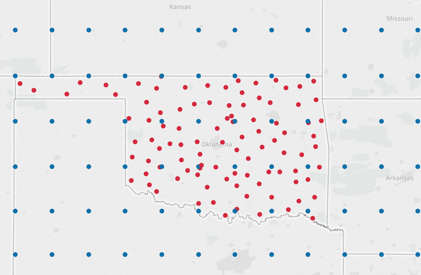
In simple terms the goal is to use the blue dots (weather forecast data) to predict the red dots (solar energy).

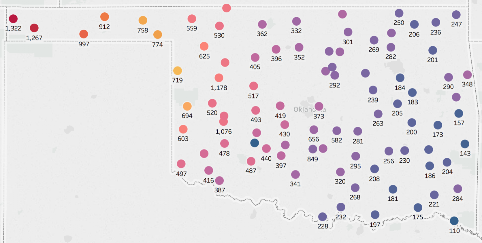
Before we do a full blown prediction let’s look at the elevation and solar energy predicted.

Station mesonets by elevation in feet.

Station mesonets by average solar energy production.

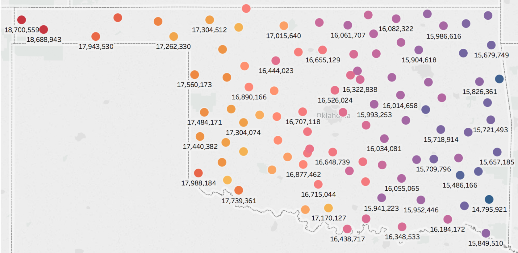
Interestingly before we have done any prediction there appears to be a relationship between elevation and solar energy production. In the southeast elevation is lower and as you move towards the northwest elevation increases. The same trend holds true for solar energy production.

Modelling, Machine Learning and Evaluation

Before we try and predict solar energy across the entire data set the approach we will use is to predict solar energy at one station for one year. Once we get all the models running we can expand to the rest of the period and stations. In this experimental phase we will use the ACME weather station to test and train.

Prior to running the model we will standardise our data. Standardising takes all our features and centres their mean to zero. We will then split the data through a train/test split. In this data set I used a 90% train and 10% test.

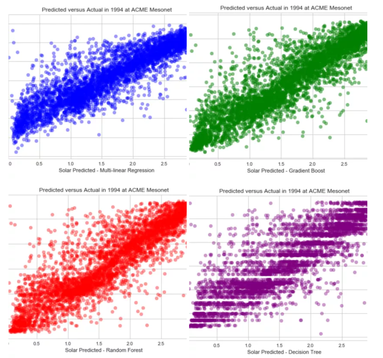
The first predictive model we will try on our data will be a simple multi-linear regression using all fifteen features as inputs. The multi-linear regression produced an r-squared of 77%. Based on just a straight multi-linear regression this is a pretty high baseline score. When we run other machine learning models using the sci-kit learn module in python we get the following cross validated results:

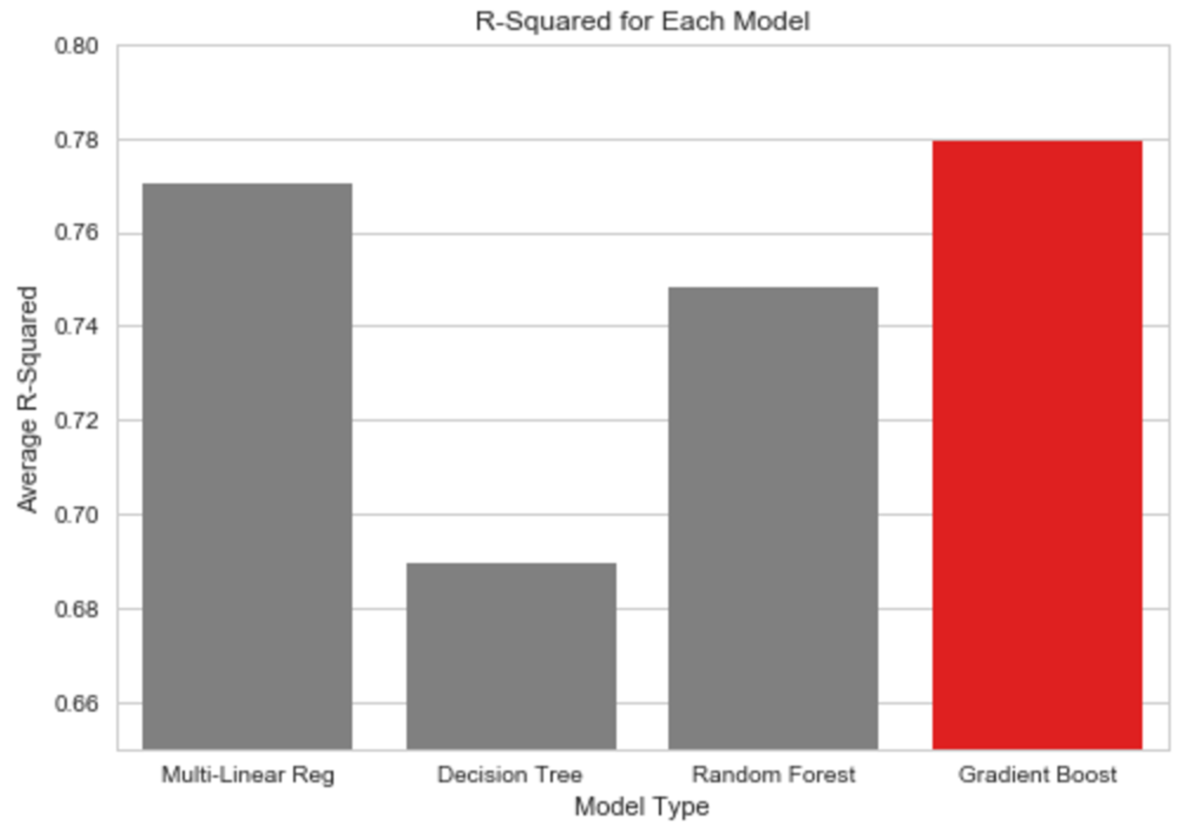
Gradient boosting method resulted with the best r-squared of 78%.

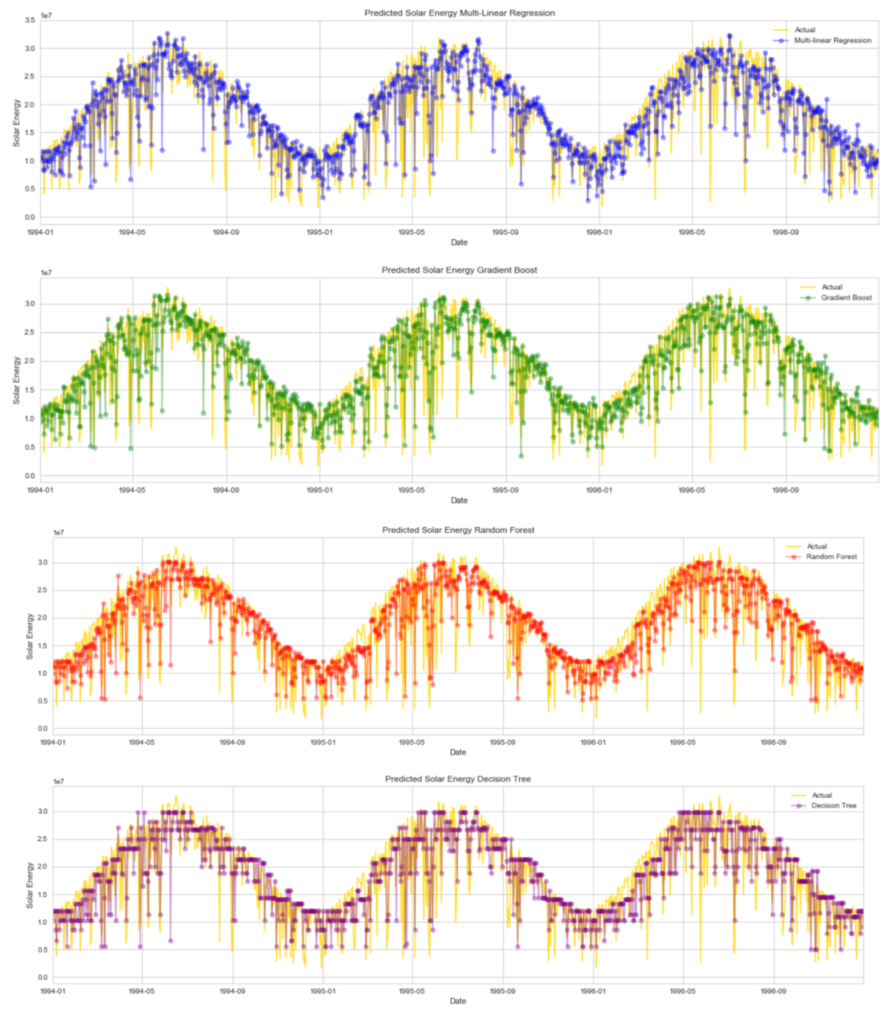
When viewing the predicted versus actual plots we can see that gradient boosting is performing the best because most the points are concentrated on the centre line with only a few points scattered . With the multi-linear regression we see more outliers and a much ‘thicker’ band down the centre line suggesting less accuracy. Whilst random forest and decision tree produce satisfactory results they both performed well below gradient boosting method. Notice that in all

models they each struggle in the 5,000,000 – 10,000,000 J/m2 which suggests that there is an underlying feature in the data.

Now that we have established a method to predict solar energy we can modify the code to propagate each model through to all stations over the fourteen year time period.

When we view the each prediction model over time we start to see the strengths of the gradient boost method. It really comes into its own at the high end of the solar energy prediction where the other models tend to under predict, especially random forest and decision tree.

Model Tuning

So now that we have established a way to predict we can now focus on tuning the model and possibly improving the efficiency of the running time. One of the benefits of gradient boosting is that it allows flexibility in tuning of the hyper parameters. When we first ran the model we used the default input parameters. Now let’s a grid search to evaluate if we can tune the parameters to output a better result. Based on some online research and discussion forums most users suggest that the following hyper parameters have the greatest impact on the gradient boost method:

1. learning_rate: range [0.05,0.08,0.11,0.14,0.17,0.2]
2. min_samples_split range [25,35,45,55]
3. min_samples_leaf range [25,50,75]
4. n_estimators range [50,100,150]
5. max_depth range [4,6,8,10]

To run the grid search fitting five folds with the above input parameters for each of 864 candidates, totalling 4320 fits. The total time taken to run the grid search was 277 seconds (4.6 minutes). Based on the input parameters the best parameters to use were:

Gradient Boost Hyper Parameters

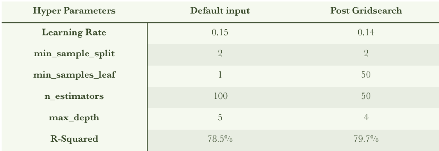
Based on the grid search tuning we improved the r-squared by 1.2%.

Now that we have tuned our hyper parameters we can perform principal component analysis (PCA). Through PCA we can evaluate if there is any opportunity at reducing dimensionality. Doing so could lead to better prediction results and reduced computing time. Using the principal component module in sci-kit learn we convert our fifteen features into principal component space. Once all our features were in the PC space we plotted the explained variance ratio versus each component to identify which ones were the major contributors. Below is the elbow plot of the each component:

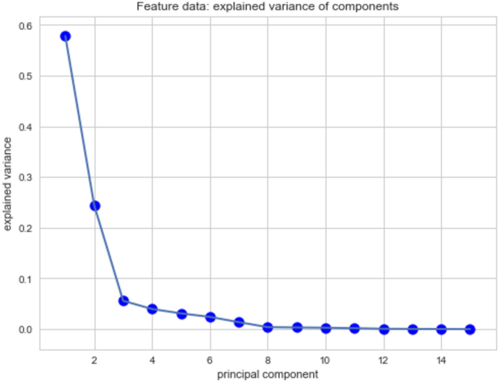
The plot above indicates that the major components are PC1, PC2 and PC3 where PC4 – PC15 explain less than one percent of all the components. Now lets see if we can see if there any major features in each component that are driving the result:

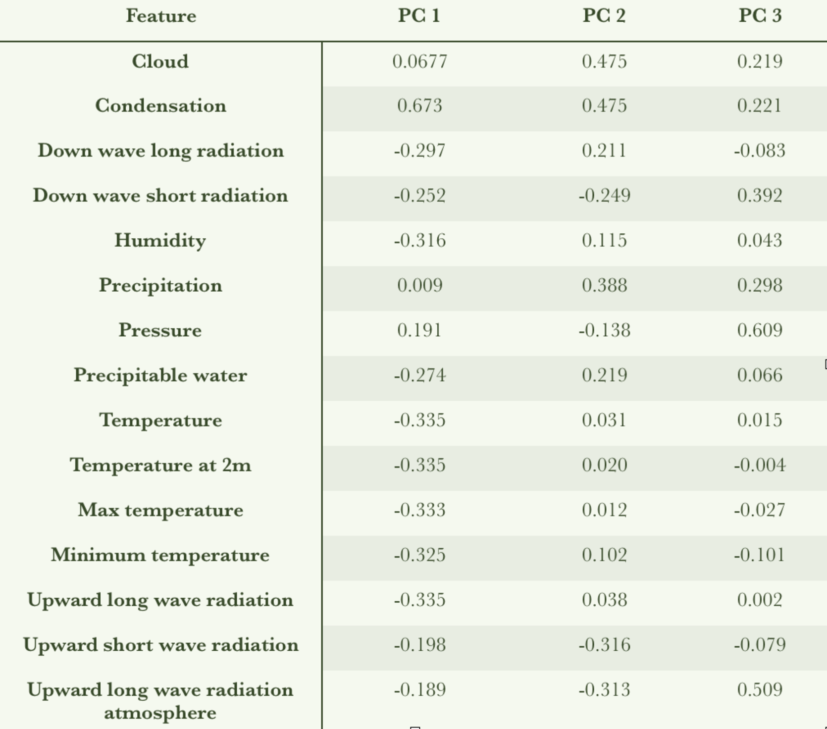
Comparing the values within each component to the features does not indicate any dominant features. This is also displayed on a scatter plot to see if there are any dominant trends in each component:

Full Scale Model Run and Processing

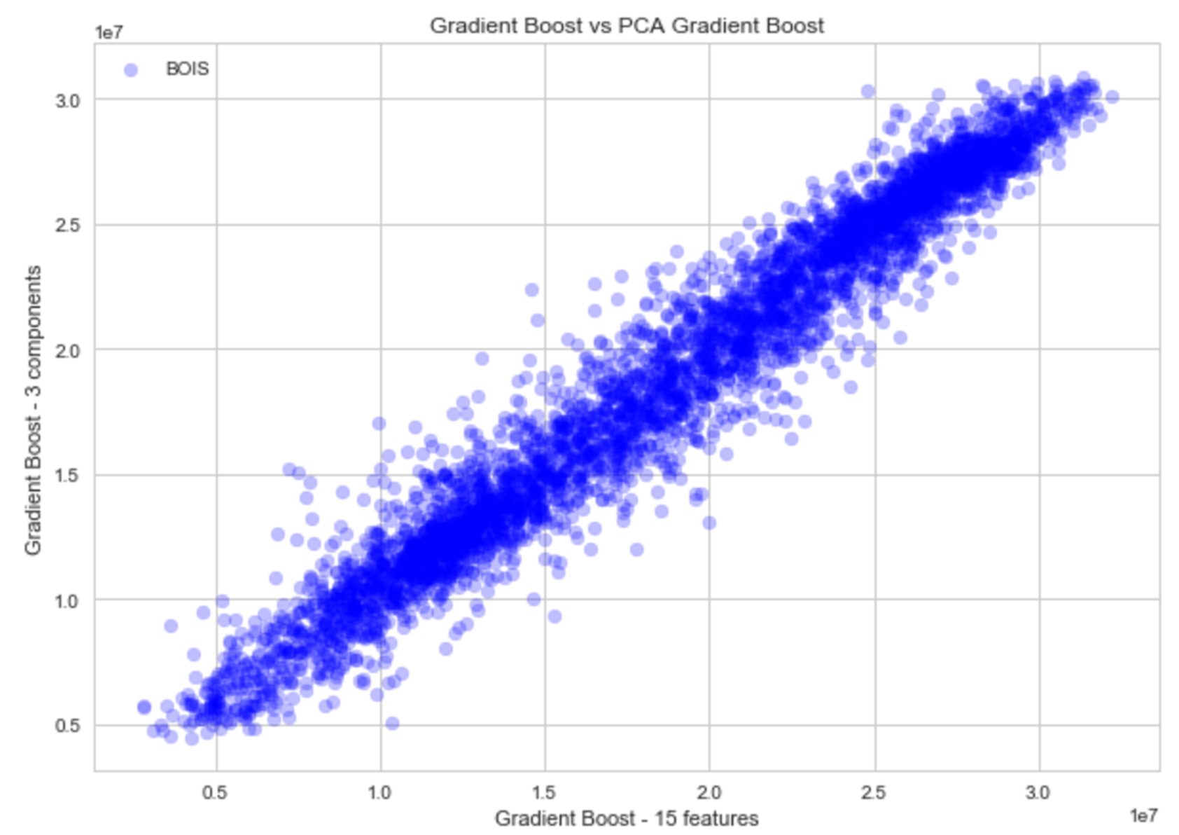
In the interest of science we are going to run all the models so we can evaluate and compare the results. If this were deployment I would choose the best two and compare. We performed two full scale runs. The first run looped through each station over the entire fourteen year period using a 90% train, 10% test split. This model did not utilise any tuning or PCA. The total run time of this model was 1475 seconds (24.6 minutes). The second run utilised the grid search input parameters and the reduced dimensionality from the principal component analysis. The total computing time for the second model run was 1087s (18.1 minutes) which is equivalent to 26% savings in time (6.5 minutes). Whilst this is not a large absolute time the PCA has the potential to save a lot if we were evaluating a larger region like the entire USA. As a check to ensure that we are not losing accuracy with the reduced dimensionality we plotted the gradient boost with 15 features versus PC reduced gradient boost. The plot below demonstrates very little loss.

A closer view of the model predictions indicate that each model struggles to predict at the high end. One possible cause is the effect of severe weather patterns like tornadoes.

Discussion & Recommendations

Gradient boosting method resulted in the best model prediction. Using PCA we were able to reduce the dimensionality from fifteen to three resulting in a 26% savings in computing time. The time savings could be significant in the commercial space if we were evaluating a larger area like the entire USA. Unfortunately when we looked at each principal component we were unable to identify the major contributing features so as an input we still require all fifteen features.

Gridsearching was used on the gradient boost method to tune the hyper parameters which resulted in a 1% improvement. If we had unlimited computing we could incorporate gridsearching for each station and use the best parameters to yield the best score however this would result in excess computing time. For example, under current computing specs the estimated run time incorporating grid searching all 98 stations would be approximately 8 hours.

Whilst multi-linear regression yields a similar r-squared it is largely affected by severe weather which reduces the accuracy of the regression.

Future Recommendations

Since forecast data is in time we could try time series prediction, however it is likely that time series prediction would only provide accurate forecasting unto one week in advance.

To further fine tune this model we could potentially look at dividing the data set up into seasons. This would potentially reduce the range of the prediction and improve the accuracy. We could also look at a severe weather identifier. Oklahoma is prone to tornadoes which are severe low pressure systems. Using the pressure data as a cutoff we could identify tornadoes and train two seperate models based on ‘normal’ weather and ‘severe’ weather. By removing the severe weather data we may be better able to predict the peak solar production because the current model struggles at the high end of the solar energy prediction. I suspect that its the tornadoes that are bringing the prediction down.

Another method would be to try deep learning on the model to see if we could improve the result even more.

Deployment

Recall that during the EDA we identified that there was a correlation between elevation and solar production. So the best location for a solar farm based purely on solar production would be the area with the highest elevation which is the northwest corner of Oklahoma. Of course this does not take into account surface infrastructure constraints and requirements.

If we were to take into account surface requirements then this project turns into an optimisation project where solar production would be another input.

As a test it would be interesting to apply this model to another geographic area to see how it performs (for example, California or even Australia).

If deploying this model on a commercial scale I would choose PCA gradient boosting and multi-linear regression. Eliminating the other two models would save further in computational time. Gridsearching each station is not really a commercial solution for the incremental gain.

Possible scenarios for further tuning and re-training involve splitting the time frame into seasons and build gradient boosting model for each season. The weather patterns would possibly be more consistent and easier to train in each season. We could also incorporate a ‘severe weather’ identifier.

From an energy company perspective I assume the goal would be to have consistent production. The priority would be to choose a solar farm location least affected by severe weather and closest to surface infrastructure. Avoiding severe weather patterns will cause fewer power interruptions.

Attempting to try the model prediction in Australia would also be intriguing.

Conclusion

• Machine learning for solar prediction works.
• Gradient boosting had best result yielding an average r-squared of 78%.
• Tuning in GB resulted in an improvement of 1.2% on the r-squared score.
• PCA reduced dimensionality and computing time by 25%
• All models struggled to predict at the top end. Possibly due to severe weather bring the forecast down.
• Elevation and solar energy are correlated. Higher elevation equals higher solar energy. Based on Oklahoma map northwest corner is best. This does not account for any surface restrictions or infrastructure and towns.
• For commercial use my recommendation would be to choose an area that has the most consistent solar production with fewest severe weather events. This would yield lower service interruptions.
• Future re-training and improvement might involve splitting the data by season and incorporating a ‘severe weather’ identifier.
• Try using deep learning to see if that would improve the prediction even greater.
• Perform solar prediction in Australia.

To view my full notebook click here to see the full notebook.